Python module

Follow the steps outlined in _installation, in order to be able to use VelocityConversion as a Python module. Start with importing the main class:

In [1]: from VelocityConversion import MantleConversion

In [2]: MC = MantleConversion()

Input data

The input data can be loaded from a file or provided as a numpy array. The data should be organised in columns:

Column

Name

Description

Unit

0

X

A coordinate

Anything

1

Y

A coordinate

Anything

2

Z

Depth

masl

3

v

Velocity

m/s

To load data from a file, use LoadFile().

In [3]: MC.LoadFile('../../Examples/VsSL2013.dat')
Loading input file: ../../Examples/VsSL2013.dat
> Velocity scale factor is 1.0

Alternatively, the data can be provided as a numpy array using LoadArray(). When providing the data as a numpy array, it should have the shape [nrows, 4]. This example shows the numpy array structure by simply displaying the array loaded from the file above:

# Adjust numpy just for some prettier printing of the array
In [4]: np.set_printoptions(precision=2, suppress=True)

In [5]: MC.DataRaw
Out[5]: 
array([[      0.  , 6000000.  ,  -50000.  ,    4287.65],
       [ 100000.  , 6000000.  ,  -50000.  ,    4268.31],
       [ 200000.  , 6000000.  ,  -50000.  ,    4199.97],
       ...,
       [1000000.  , 7800000.  , -200000.  ,    4329.93],
       [1100000.  , 7800000.  , -200000.  ,    4338.  ],
       [1200000.  , 7800000.  , -200000.  ,    4352.14]])

In any case, the velocity type needs to be provided with SetVelType() (S or P):

In [6]: MC.SetVelType('S')

Defining a mantle assemblage

The mineralogical assemblage of the mantle rocks must be provided. The assemblage is defined by denoting the fractional proportion of a mineral phase of the mantle rock. It can be defined either by using a Python dictionary, or loaded from a file using LoadMineralogy():

In [7]: assemblage = {
   ...:     "ol": 0.67,
   ...:     "cpx": 0.045,
   ...:     "opx": 0.225,
   ...:     "gnt": 0.06,
   ...:     "XFe": 0.11
   ...: }
   ...: 

Note

XFe is the molar iron content of the rock and is optional. It can also be defined by calling SetXFe().

The available mineral phases are provided in the MinDB.csv. This file can be edited freely if new phase information is available.

To defined the composition, call SetMineralogy():

In [8]: MC.SetMineralogy(assemblage)
> XFe assigned to 0.11
> All mineral phases are known
> Sum of mineral phases equals 1.0

or call DefaultMineralogy() in order to set the default composition (garnet lherzolite by Jordan, 1979).

Start the conversion

To start the conversion, simply run Convert():

In [9]: MC.Convert()
Filling tables
> Number of depth values: 5
> Number of temperatures: 2701
> Pressure calculation  : AK135
> T range: 300.0 to 3000.0 steps 1.0
Starting temperature estimation
> Progress: 0%
> Progress: 0%
> Progress: 20%
> Progress: 40%
> Progress: 60%
> Progress: 100%
> Done!

Results

The results are stored in two 1D arrays named Result_T and Result_Rho. The order of the data in these arrays corresponds to the order of the points in the input file.

In [10]: print(MC.Result_T)
[1288.78 1301.07 1341.16 ... 1552.29 1546.6  1536.44]

In [11]: print(MC.Result_Rho)
[3311.46 3310.48 3307.29 ... 3407.16 3407.53 3408.18]

Warning

The temperatures in Result_T are in Kelvin!

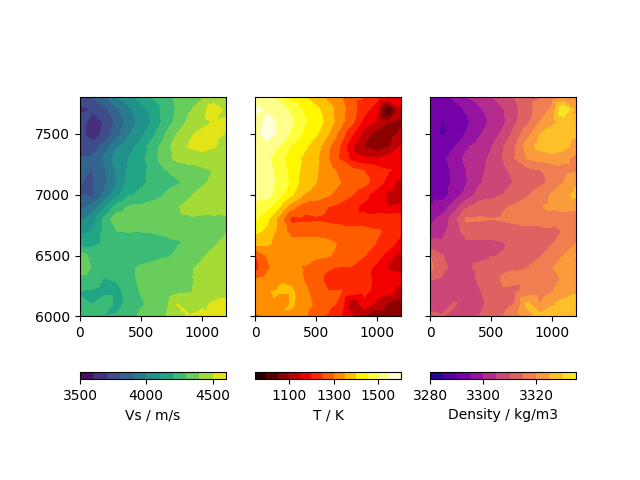
We can plot the results for 50km depth:

In [12]: import matplotlib.pyplot as plt
   ....: from matplotlib.tri import Triangulation
   ....: 
   ....: def make_plot(MCObject, depth):
   ....:     fig, ax = plt.subplots(1, 3, sharex=True, sharey=True)
   ....:     indices = MCObject.DataRaw[:, 2] == depth
   ....:     depth_slice = MCObject.DataRaw[indices]
   ....:     velocity = depth_slice[:, 3]
   ....:     temperature = MCObject.Result_T[indices]
   ....:     density = MCObject.Result_Rho[indices]
   ....:     tri = Triangulation(depth_slice[:, 0]/1000.,
   ....:                         depth_slice[:, 1]/1000.)
   ....:     m_v = ax[0].tricontourf(tri, velocity, levels=np.arange(3500, 4700, 100))
   ....:     m_t = ax[1].tricontourf(tri, temperature, cmap='hot', levels=np.arange(950, 1650, 50))
   ....:     m_d = ax[2].tricontourf(tri, density, cmap='plasma', levels=np.arange(3280, 3340, 5))
   ....:     for a in ax:
   ....:         a.set_aspect('equal')
   ....:     fig.colorbar(m_v, ax=ax[0], label='Vs / m/s', orientation='horizontal',
   ....:                  ticks=[3500, 4000, 4500])
   ....:     fig.colorbar(m_t, ax=ax[1], label='T / K', orientation='horizontal',
   ....:                  ticks=[1100, 1300, 1500])
   ....:     fig.colorbar(m_d, ax=ax[2], label='Density / kg/m3', orientation='horizontal',
   ....:                  ticks=[3280, 3300, 3320, 3340])
   ....: 

In [13]: make_plot(MC, -50e3)

Saving to file

The results can be saved to an output file with SaveFile():

In [14]: MC.SaveFile('fileout.dat')
Saving results to fileout.dat
> Done!

The output file will contain metadata about the conversion parameters, for example:

# Temperature output
# Input file: VsSL2013.dat
# Velocity scale factor: 1.0
# Mantle composition:
# cpx - 0.133
# gnt - 0.153
# jd - 0.045
# ol - 0.617
# opx - 0.052
# XFe - 0.11
# Pressure calculation: AK135
# Wave frequency (Omega) / Hz: 0.02
# Anelasticity parameters: Sobolev et al. (1996)
# Alpha depending on: Nothing
# Columns:
# 1 - X
# 2 - Y
# 3 - Z / masl
# 4 - V_S / m/s
# 5 - T_syn / degC
# 6 - Rho / kg/m3

Optional settings

Pressure reference model

Pressure in VelocityConversion is computed one-dimensionally using the earth reference model AK135. If desired, pressure calculation can be performed using a homogeneous density. Therefore, define

In [15]: MC.SimpleP = True

In [16]: MC.SimpleRho = 3000.  # kg/m3, the default value

If pressure was computed in this way, a note in the output metadata will be added:

# Pressure calculation: Simplified
# Pressure calculation density: 3000.0 kg/m3

Attenuation parameters

The attenuation model used can be changed. By default, parameterisation after Sobolev et al. (1996) is used. If desired, it can be changed to the parameters by Berckhemer et al. (1982) using SetQMode():

In [17]: MC.SetQMode(1)  # Sobolev et al. (1996)
Using Q after Sobolev et al. (1996)
    a = 0.15
    A = 0.148
    H = 500000.0 J/mol
    V = 2e-05 m3/mol

In [18]: MC.SetQMode(2)  # Berckhemer et al. (1982)
Using Q after Berckhemer et al. (1982)
    a = 0.25
    A = 0.0002
    H = 584000.0 J/mol
    V = 2.1e-05 m3/mol

Thermal expansion coefficients

Goes et al. (2000) use a temperature-dependent isobaric thermal expansion coefficient. In general, the expansion coefficient will increase with increasing pressure. However, the expansion coefficient is also sensitive to pressure changes such that it will decrease with increasing pressure. Temperature and pressure act against each other. I therefore implemented three different options to use this expansion coefficient. They are defined using SetAlpha():

`mode`	Explanation
const	Constant. Use \(\alpha_0\) of Saxena and Shen (1992)
T	T-dependent. Use the formulation of Saxena and Shen (1992)
PT	Pressure- and temperature dependent. Uses data extracted from Hacker and Abers (2006)

The temperature dependent alpha is defined by

\[\alpha(T) = \alpha_0 + \alpha_1 T + \alpha_2 T^{-1} + \alpha_3 T^{-2}\]

Where the parameters \(\alpha_i\) are taken from Saxena and Shen (1992). They are provided in the file MinDB.csv.

The data for pressure and temperature dependent behaviour were extracted from the Excel worksheet by Hacker and Abers (2006) using a VBA script.

The following figure shows how the expansion coefficients compare for clinopyroxene (cpx):

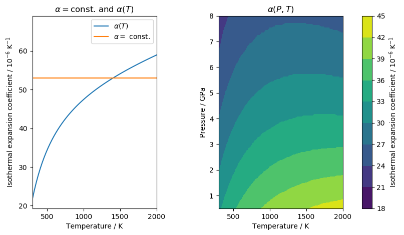
In [19]: MC.SetAlpha('const')