Computations
Thermal field
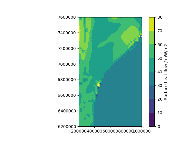
Surface heat flow
pyGMS can compute and plot the surface heat flow using
compute_surface_heat_flow() and
plot_surface_heat_flow(). When calling the plot
method, pyGMS will automatically compute the heat flow if it has not been
computed beforehand:
In [1]: from pyGMS import GMS
...: import matplotlib.pyplot as pl
...: from matplotlib import tri
...: model = GMS('../../examples/model.fem')
...: model.layer_add_var('T')
...:
Loading ../../examples/model.fem
Done!
Triangulating layers
Done!
In [2]: fig, ax = plt.subplots()
...: ax.set_aspect('equal')
...: cm = model.plot_surface_heat_flow(ax=ax, levels=np.linspace(0, 80, 9))
...: fig.colorbar(cm, ax=ax, label='Surface heat flow / mW/m2');
...:
������������������������������������������������������������������Computing surface heat flow
Rheology
If the model contains temperatures, pyGMS can compute the rheological behaviour based on fixed background strain rates.
Note
Make sure to use a model with refined surfaces in order to obtain valid results!
Definition of rheological properties
The rheological properties within pyGMS must be provided as a list of dictionaries. Each of the dictionaries contains the properties for one rock type. The keys of rock property dictionaries can be as follows:
Key
Description
Unit
Byerlee’s law
f_f_e
Friction coefficient for extension
–
f_f_c
Friction coefficient for compression
–
f_p
Pore fluid factor
–
rho_b
Bulk rock density
kg/m3
Dislocation creep
a_p
Pre-exponential scaling factor
Pa^(-n)/s
n
Power law exponent
–
q_p
Activation energy
J/mol
Diffusion creep
a_f
Pre-exponential scaling factor
1/Pa/s
q_f
Activation energy
J/mol
d
Grain size
m
m
Grain size exponent
–
Dorn’s law properties
sigma_d
Dorn’s law stress
Pa
q_d
Dorn’s law activation energy
a_d
Dorn’s law strain rate
The following example shows how a list of materials is defined for the model loaded above:
In [3]: materials = list()

In [4]: materials.append(dict(name='quartzite_wet_2440',
   ...:         # Byerlee's law
   ...:         f_f_e=0.75,       # Friction coefficient extension
   ...:         f_f_c=2.0,        # Friction coefficient compression
   ...:         f_p=0.35,         # Pore fluid factor
   ...:         rho_b=2440.0,     # Bulk density
   ...:         # Dislocation creep
   ...:         a_p=1e-28,        # Preexponential scaling factor
   ...:         n=4.0,            # Power law exponent
   ...:         q_p=223e3))       # Activation energy
   ...:

In [5]: materials.append(dict(name='quartzite_wet_2800',
   ...:         # Byerlee's law
   ...:         f_f_e=0.75,       # Friction coefficient extension
   ...:         f_f_c=2.0,        # Friction coefficient compression
   ...:         f_p=0.35,         # Pore fluid factor
   ...:         rho_b=2800.0,     # Bulk density
   ...:         # Dislocation creep
   ...:         a_p=1e-28,        # Preexponential scaling factor
   ...:         n=4.0,            # Power law exponent
   ...:         q_p=223e3))       # Activation energy
   ...:

In [6]: materials.append(dict(name='diabase_dry',
   ...:         altname='Gabbroid rocks',
   ...:         # Byerlee's law
   ...:         f_f_e=0.75,       # Friction coefficient extension
   ...:         f_f_c=2.0,        # Friction coefficient compression
   ...:         f_p=0.35,         # Pore fluid factor
   ...:         rho_b=2800.0,     # Bulk density
   ...:         # Dislocation creep
   ...:         a_p=6.31e-20,     # Preexponential scaling factor
   ...:         n=3.05,           # Power law exponent
   ...:         q_p=276.0e3))     # Activation energy
   ...:

In [7]: materials.append(dict(name='plagioclase_wet',
   ...:         # Byerlee's law
   ...:         f_f_e=0.75,       # Friction coefficient extension
   ...:         f_f_c=2.0,        # Friction coefficient compression
   ...:         f_p=0.35,         # Pore fluid factor
   ...:         rho_b=3100.0,     # Bulk density
   ...:         # Dislocation creep
   ...:         a_p=3.981e-16,    # Preexponential scaling factor
   ...:         n=3.0,            # Power law exponent
   ...:         q_p=356e3))       # Activation energy
   ...:

In [8]: materials.append(dict(name='peridotite_dry',
   ...:         # Byerlee's law
   ...:         f_f_e=0.75,       # Friction coefficient extension
   ...:         f_f_c=2.0,        # Friction coefficient compression
   ...:         f_p=0.35,         # Pore fluid factor
   ...:         rho_b=3300.0,     # Bulk density
   ...:         # Dislocation creep
   ...:         a_p=5.011e-17,    # Preexponential scaling factor
   ...:         n=3.5,            # Power law exponent
   ...:         q_p=535e3,        # Activation energy
   ...:         # Diffusion creep
   ...:         a_f=2.570e-11,    # Preexp. scaling factor
   ...:         q_f=300e3,        # Activation energy
   ...:         d=0.1e-3,         # Grain size
   ...:         m=2.5,            # Grain size exponent
   ...:         # Dorn's law
   ...:         sigma_d=8.5e9,    # Dorn's law stress
   ...:         q_d=535e3,        # Dorn's law activation energy
   ...:         a_d=5.754e11))    # Dorn's law strain rate
   ...:
These properties can then be linked to the layers using
set_rheology():
In [9]: body_materials={
   ...:     'Sediments':'quartzite_wet_2440',
   ...:     'UpperCrustPampia': 'quartzite_wet_2800',
   ...:     'UpperCrustRDP': 'diabase_dry',
   ...:     'LowerCrust':'plagioclase_wet',
   ...:     'LithMantle': 'peridotite_dry',
   ...:     'Base':'peridotite_dry'
   ...: }
   ...:

In [10]: strain_rate = 1e-16   # Strain rate in 1/s

In [11]: model.set_rheology(strain_rate, materials, body_materials)
Note
There may be much more materials listed in materials than referred to
in body_materials.
Yield strength envelopes
In order to plot a yield strength envelope, use the
plot_yse() method. The method requires a location
loc which may either be a Well or a coordinate:
In [12]: x = 400e3
   ....: y = 7400e3
   ....: loc = (x, y)
   ....: kwds_fig = {'figsize': (5, 5), 'dpi': 75}
   ....:

In [13]: model.plot_yse(loc, plot_bodies=True, kwds_fig=kwds_fig);
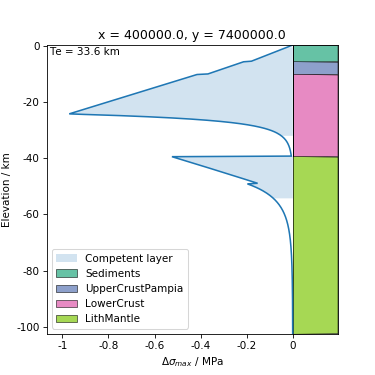
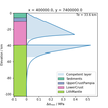
By default, the envelopes for compression are displayed. This can be changed
using the mode argument:
In [14]: model.plot_yse(loc, mode='extension', plot_bodies=True, kwds_fig=kwds_fig);
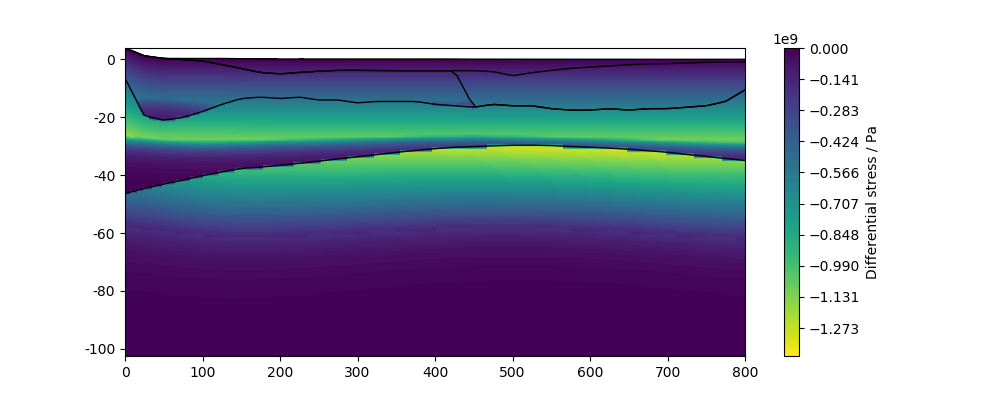
Yield strength profiles
Yield strength profiles are colour-coded yield strength envelopes in profile
view. They can be plotted with the
plot_strength_profile() method.
In [15]: x0 = 200e3
   ....: y0 = 7000e3
   ....: x1 = 1000e3
   ....: y1 = 7000e3
   ....:

In [16]: fig, ax = plt.subplots(figsize=(10,4))
   ....: color_levels = np.linspace(-1.4e9, 0, 100)
   ....: cm = model.plot_strength_profile(x0, y0, x1, y1, ax=ax,
   ....:                                  levels=color_levels)
   ....: model.plot_layer_bounds(x0, y0, x1, y1, ax=ax)
   ....: fig.colorbar(cm, ax=ax, label='Differential stress / Pa');
   ....:
Computing strength
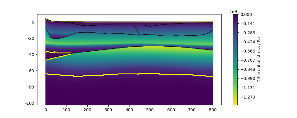
Wit pyGMS you can also plot the extent of the competent layers using the
show_competent=True argument. The thicknesses of the competent layers are
determined following the method proposed by
Burov and Diament (1995).
In [17]: fig, ax = plt.subplots(figsize=(10,4))
   ....: kwds_competent = dict(color='yellow')
   ....: cm = model.plot_strength_profile(x0, y0, x1, y1, ax=ax,
   ....:                                  levels=color_levels,
   ....:                                  show_competent=True,
   ....:                                  competent_kwds=kwds_competent)
   ....: model.plot_layer_bounds(x0, y0, x1, y1, ax=ax)
   ....: fig.colorbar(cm, ax=ax, label='Differential stress / Pa');
   ....:
Computing strength
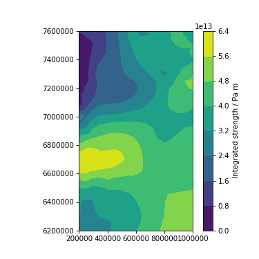
Integrated strength
The integrated strength is computed with the
compute_integrated_strength() method. The strength
is then stored as numpy array within the variable integrated_strength. Note
that the computation of the integrated strength is time consuming as Python
needs to iterate through many wells within the model:
In [18]: model.compute_integrated_strength(spacing=50e3)
Computing integrated strength
It needs to be plotted individually:
In [19]: strength = model.integrated_strength
   ....: triangulation = tri.Triangulation(strength[:, 0], strength[:, 1])
   ....: fig, ax = plt.subplots(figsize=(5,5), dpi=75)
   ....: ax.set_aspect('equal')
   ....: cm = ax.tricontourf(triangulation, strength[:, 2])
   ....: fig.colorbar(cm, label='Integrated strength / Pa m');
   ....:
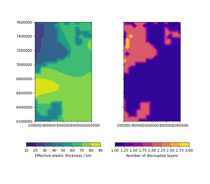
Effective elastic thickness
The effective elastic thickness can be computed with pyGMS using the
compute_elastic_thickness() method. If no strain
rate is explicitely given, it will use one that was defined earlier.
In [20]: model.compute_elastic_thickness(dx=50e3)
Computing elastic thickness
> Mode                      : compression
> Strain rate               : 1e-16 1/s
> Horizontal resolution     : 50000.0 m
> Number of vertical points : 500
> Min. sigma criterion      : 20 MPa
> Lithostatic pressure crit.: 5.0 % of Plitho
The results are stored in the variable elastic_thickness. This variable
consists of two arrays: the number of decoupled layers (1D array), and the
array for the effective elastic thickness (2D array).
Plotting the elastic thickness next to the number of decoupled layers:
In [21]: nlays, eet = model.elastic_thickness[strain_rate]
   ....: triangulation = tri.Triangulation(eet[:, 0], eet[:, 1])
   ....:

In [22]: fig, ax = plt.subplots(1, 2, sharex=True, sharey=True,
   ....:                        figsize=(8, 7))
   ....: ax[0].set_aspect('equal')
   ....: ax[1].set_aspect('equal')
   ....: cm_eet = ax[0].tricontourf(triangulation, eet[:, 2]/1000)
   ....: cm_nlay = ax[1].tricontourf(triangulation, nlays, cmap='plasma')
   ....: fig.colorbar(cm_eet, ax=ax[0], orientation='horizontal',
   ....:             label='Effective elastic thickness / km')
   ....: fig.colorbar(cm_nlay, ax=ax[1], orientation='horizontal',
   ....:             label='Number of decoupled layers');
   ....:
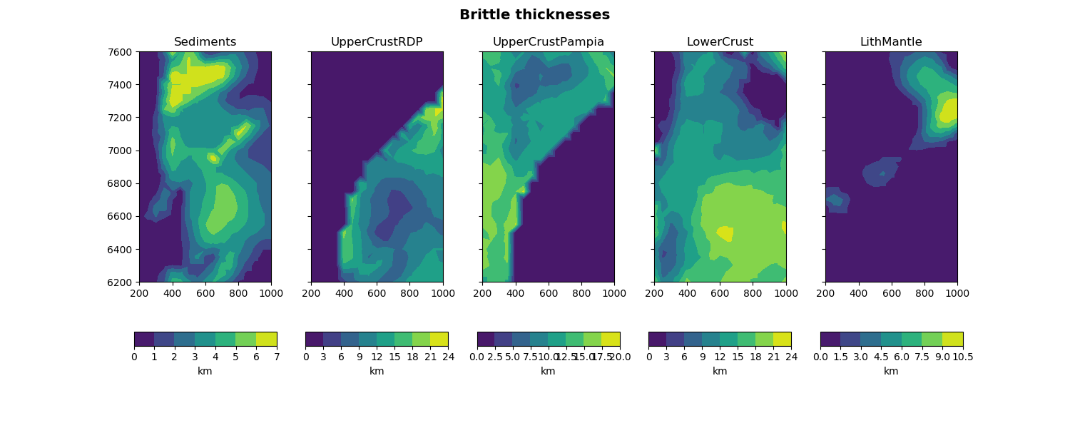
Brittle-ductile transition
pyGMS can compute the thicknesses of brittle and ductile zones for each layer
using the compute_bd_thickness() method. The
results are stored in the variables t_ductile and t_brittle. These
variables are list of length 3, with this structure:
t_ductile = [
    list(x),                    # x-coordinates / m
    list(y),                    # y-coordinates / m
    dict(layer_id : t_ductile)  # brittle or ductile thickness / m
]
In this example, we compute the brittle/ductile thicknesses of the layers and create a plot showing the brittle thicknesses of all layers in km:
In [23]: model.compute_bd_thickness(dx=50e3)
Computing brittle/ductile thicknesses
> Strain rate: 1e-16 1/s
> Resolution : 50000.0 m

In [24]: x = model.t_brittle[0]/1000
   ....: y = model.t_brittle[1]/1000
   ....: ts = model.t_brittle[2]
   ....:

In [25]: triangles = tri.Triangulation(x, y)
   ....: fig, axes = plt.subplots(1, len(ts.keys()) - 1,
   ....:                         sharex=True, sharey=True,
   ....:                         figsize=(15,6))
   ....: fig.suptitle('Brittle thicknesses', fontweight='bold', fontsize='x-large')
   ....: i = 0
   ....: for layer_id in ts:
   ....:     if layer_id == model.n_layers - 1:
   ....:         break
   ....:     layer_name = model.layer_dict[layer_id]
   ....:     ax = axes[i]
   ....:     ax.set_aspect('equal')
   ....:     cm = ax.tricontourf(triangles, ts[layer_id]/1000)
   ....:     ax.set_title(layer_name)
   ....:     fig.colorbar(cm, ax=ax, orientation='horizontal', aspect=10, label='km')
   ....:     i += 1
   ....: